How do you find your top 3 favorite Disney movies?
What is the problem?
How would you find your top 3 favorite Disney movies? Even if you were to consider just the movies from the last 10 years, that’s a lot of movies to consider (an even 100 as of writing this post).
If this question were asked in a programming environment, we would probably use quick-sort easy-peasy since it’s pretty fast with an average runtime of \(\mathcal{O}(n\log{}n)\). However, if this were asked in a human environment (strange, I know), quick sort may not be the best since the worst case number of comparisons is \(\mathcal{O}(n^2)\). For example, if we were working with 100 Disney movies, then in the worst case, we would have to ask “Which do you like better: movie X or movie Y” 10,000 times. At that point, you would probably prefer a faster but less accurate format, maybe a Buzzfeed article?
Solutions
Solution 1 - Sort the entire list
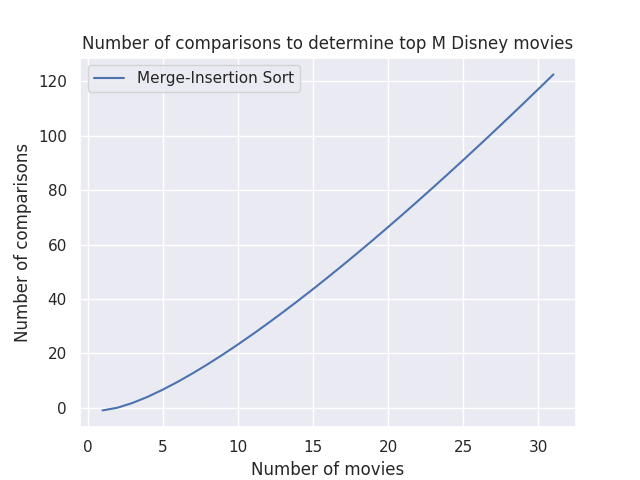
If we choose to sort the entire list, we’re better off using a sorting algorithm that uses the least number of comparisons, which according to Wikipedia is merge-insertion sort. Using merge-insertion sort, we can sort the entire list with approximately \(n\log{}n - n\) comparisons.
 |
|---|
| Fig. 1 - Merge-insertion sort comparisons |
The number of comparisons goes up pretty quickly as the number of movies increases. If we had a small number of movies, this would probably work ok but not so good if we want to consider a larger input size.
Solution 2 - Keep a top \(M\), sorted buffer
If we are only looking for the top 3 movies, we just need to keep a sorted buffer of size 3. The rest, we can discard since they are not relevant. This reduces the total number of comparisons greatly. In the average case, we’ll be doing \(\mathcal{O}(n\log{}m)\) comparisons where \(n\) is the total number of items you’re considering and \(m\) is the number of items in your “top” list.
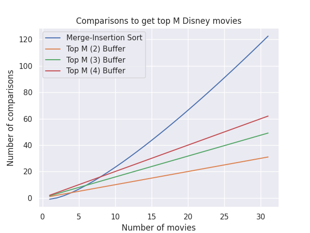
With the buffer approach, we no longer need to sort the entire list. We just need to keep track of the top \(M\) movies. This reduces the number of comparisons from \(n\log{}n - n\) from Solution 1 to \(n\log{}m\).
 |
|---|
| Fig. 2 - TopM comparisons |
The topM solution works pretty good as long as our \(M\) is reasonably small. The larger the \(M\), the more comparisons.
Solution 3 - Create a tier list
With many sorting algorithms, either the entire list is sorted or it isn’t. If we want to incrementally sort a dataset, one idea that we could do is to first split the input list into various buckets, similar to radix sort. By creating different tiers, we get a few benefits:
- Prune the input list so that we don’t have to process as many elements when it comes time to comparing the movies directly
- Gives us the option to incrementally sort the remaining list without iterating over the entire remaining list
After categorizing the movies into these buckets, we can move forward and run solution 2 to create a buffer to determine our top \(M\) favorite movies.
This approach may work but I don’t know how much value we get from initially sorting items into buckets and then.
By bucketing the different items into buckets, we’ve pruned our input list to \(1 \over b\) where \(b\) is the number of buckets. This also assumes an average distribution of items to buckets . Assuming our size of our “top” list does not span multiple buckets, the total number of comparisons is as follows: \(\mathcal{O}(n + {n \over b} * \log{}m)\). The breakdown is as follows:
- \(n\) - the number of comparisons it takes to categorize a movie into each \(b\) buckets
- \(n \over b\) - the total number of items in a given bucket. Assuming each bucket has roughly the same number of items
- \(\log{}m\) - The number of comparisons required to determine if a movie belongs in your top \(M\) movies
 |
|---|
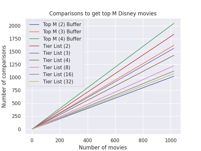
| Fig. 3 - TopM and Tier List comparisons |
This works pretty good! The only topM option that out-performs our tier list solution is topM-2. Practically speaking, it is probably not a great experience to ask the user to categorize a movie into 32 buckets but that’s a problem for another time :D
What happens if we want to find the next top \(M\) movies?
Let’s say we’ve run one of our sorting algorithms and we currently have our top \(M\) movies. What would be the cost to find the next \(M\)? Or the \(M\) after that?
 |
|---|
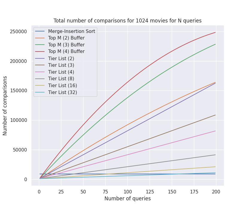
| Fig. 4 - Cumulative comparisons per query |
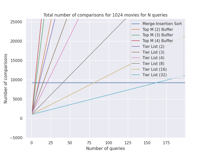 |
|---|
| Fig. 5 - Zoomed-in version of Fig. 4 |
For merge-insertion sort, the cost jumps down to 0 to find the next M movies since we had already sorted the list. As such, the merge-insertion sort line is horizontal with no additional cost for subsequent queries. Nice!
The topM performance is not so great since we are not sorting or bucketing the remainder list and have to run against \(n-m, n-2m, n-3m,…\) for each subsequent query.
The tier list behavior is interesting. The more tiers we have, the fewer comparisons we have to make for subsequent queries, which makes sense. More tiers = fewer items per tier. The best behavior I saw was with the tier list with 32 buckets. It continues to outperform the merge-insertion sort until ~162 queries.
Note: The graphs above don’t take into considertion that when we find the intial top \(M\) in the bucket for the tier-list sorts, we would not need to sort through the entire bucket again, only \(B\) - \(M\), where \(B\) is the average size of a bucket. I don’t think it would make a huge difference, it would just result in a sawtooth pattern as the number of comparisons would decrease as we continue sorting the unsorted portion of the bucket.
Conclusion
If you only need the top \(M\) movies, using the top \(M\) buffer solution (Solution 2) works well with all sizes of \(n\). If you potentially need to find the next \(P\) top \(M\) movies, using the top \(M\) solution still works provided that \(P\) is less than 5 or 6. If you need to query more than that, you’re better off using the tier list approach. In theory, the more buckets the better but in practice, it may be difficult for the user to accurately categorize a movie across 32 buckets.